
You notice some weird alerts in your environment and start to investigate them. As you’re digging into the myriad of log and monitoring data, you realize that what you’re looking at is a telltale sign of data exfiltration — you’ve had a breach.
You follow the trail and eventually realize that the breach started before the earliest retention date of your log data. You have no way of forensically proving when the breach started, or even the true scope of the breach. Adding to your distress are the growing number of data privacy laws that are requiring breach notification — as of this writing, the EU’s General Data Privacy Regulation (GDPR) requires notifications to potential victims of breaches within 72 hours of the discovery of the breach.

Optimizing for fast search carries significant costs which grow linearly with retention time.
While most companies want to retain data longer, the cost of retention is the major factor driving retention decisions. The real constraint is that many companies use indexed log management systems as their “system of record” for log information, even though there is a significant premium on those systems, because the tools don’t have efficient mechanisms for archiving and re-ingesting data. This makes them extremely expensive for retention (for more info on the cost of log management, see our Why Log Systems Require So Much Infrastructure blog post). At Cribl, we believe that there is a better way to do retention AND investigation — making it possible to retain far more data than you do now, while being able to make use of any of it, for less money than you are spending today.
First, a little history.
In 2004, when Splunk first rolled out their product, the cloud as we know it really didn’t exist yet. Back then, everything was either storage local to a server or SAN storage, and archive storage was using SATA disks instead of Fibre or SCSI disks. Those were really the only options for retention, so it made sense that the go-to strategy was to retain all data within the log analysis system.
As data volumes grew, customers started using the “frozen bucket” model. This allowed them to export data from their environment, which helped to improve performance on live data, but didn’t solve the retention problem. If you needed to pull frozen data from archives, you needed to “thaw” entire files and make them available to the system. While this wasn’t particularly difficult, it was very time consuming, and didn’t provide the capability to limit the data you were pulling in — it was everything in the “frozen” file, or nothing.
In 2006, AWS made the Simple Storage Service (S3) available, and initial pricing was about $0.15/GB per month. But because it was object storage, most of the industry didn’t directly support it, so most who used it were either running custom programs, or just using it as an archive destination to copy data to. As of 2020, S3 pricing has come down to $0.023/GB per month, and more and more software vendors have integrated the technology into their products. AWS has also expanded the service to include much cheaper archive options, like Glacier ($0.004/GB per month) or Glacier Deep Archive ($0.00099/GB per month), all still accessible via the S3 API. Other cloud providers have similar offerings, and the competition has helped drive cost down on all of them. Archiving data at scale has never been less expensive.
Cheap storage has reduced the cost of retention, but it hasn’t relieved the pain of using that data. In fact, now, instead of having archives on moderately fast SATA drives that were local to the log infrastructure, the archives were now only available via the internet (or a dedicated line). This slows down the “thawing” process even more, as you have to copy it locally first, then decompress it, before it is available for analysis.
Expanding retention.
According to a 2023 study by IBM, the average time from the occurrence of a security breach to detection is 204 days, with an additional 73 days to contain a breach. If your retention policy keeps 12 months of data around, as long as your detection stays near the average, you can readily get at data going back to the beginning of the breach. Yet beyond averages, we also hear a number of stories like the Marriott breach (which took 4 years to detect) or the Dominion National breach (which took 9 *years* to detect). So it’s clear that the retention of data critical for investigations is an important part of any security incident response plan.
Storing data in object storage could be as little as 1% of the cost of storing it online in an indexing engine.
With many companies retaining logs for just 12 to 18 months, any long-running breach will be next to impossible to work back to the beginning of the breach via logs. For the purposes of this paper, we will use a fictitious company, Sprockets, Inc. to illustrate different approaches to solving the problem.
Our company generates about 1TB of logs per day, in instances using gp2 Elastic Block Store (EBS) volumes. The monthly recurring cost (MRC) is roughly $3,000 for each month of retention. The same data, stored in Glacier Deep Archive, has an MRC of about $30.
Sprockets has a budget that allows them 12 months of retention at the EBS price, spending $36,000/month or $432,000/year. The Deep Archive approach would cost them only $360/month or $4,320/year, freeing up a lot of budget to expand retention (5 years of retention = $21,600/year, 10 years of retention = $43,200/year), and/or invest in other things.
Investigating a breach, the “old” way.
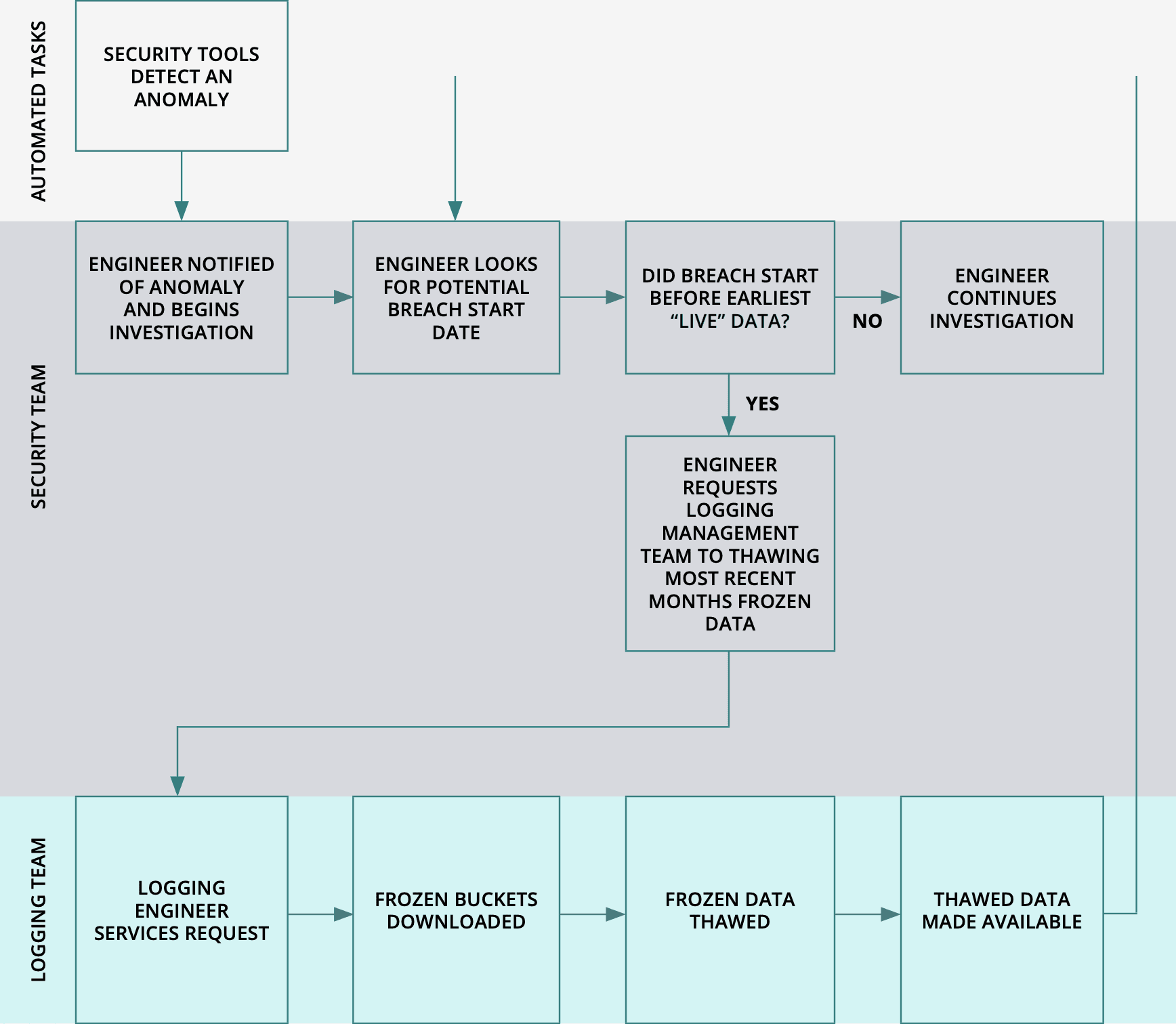
Within our fictitious company, a security tool detects an anomaly and alerts the on-call security engineer. The engineer starts digging through logs and realizes that there has been a breach, which looks to involve three servers, a firewall pair, and a switch pair. After more digging, she realizes that it started some time earlier than the earliest data in the logging system. The engineer has to ask the logging team to thaw earlier data, which has been archived in AWS S3. Because they need to retrieve all of the data for a given time window at once, the engineer requests only a month, waits for it to be present, checks it, and if the beginning of the incident is not there, has to repeat the process until the data needed is present.
Since each one of those requests is a handoff to another team member, the process slows to a crawl.
[Indexing] has been stretched to be a one-size-fits-all solution for all log data problems.
As you can see, moving your retention to “cheap storage” saves you a lot of money, but it alone does not solve the problem of getting that data back when you need it. The traditional route of pulling back the “frozen” files whole, thawing them, and attaching them to your log system would be too slow to be able to get meaningful data quickly. With many of the data privacy laws now in place and expected, the window for breach disclosure is becoming increasingly tight.
Since Sprockets does business in the EU, they need to notify anyone potentially impacted of a breach within the mandated GDPR 72-hour window. No company wants to put out a breach notification without at least an idea of when the breach started and how many customers were exposed. So it’s important to have an approach that speeds up data collection and allows you to filter data before pulling it across the wire. This approach minimizes data travel/decompress/ingestion time, which also will minimize the amount of storage and ingestion licensing you’ll need to accommodate the data.
This is where Cribl Stream comes in. Placing a Cribl Stream deployment between your logging sources and your log analytics system allows you to archive all of the data to a cheap storage mechanism for retention. This frees you up to reduce what’s going into your logging system to just what you really need day to day – via filtering unnecessary events, sampling repeating events, and cleaning up messy data. This, in turn, puts less stress on your logging system, improving performance (smaller haystacks = needles are easier to find). Stream 2.2 introduced Data Collection to the product, which enables a flexible and efficient way to retrieve data from the archive, filtering it based on the partitioning scheme of the data (more on this later).
Investigating a breach, the Stream way.
Let’s revisit our fictitious company, Sprockets. With 1TB/day of data, they’re able to install and use the free version of Stream and move their retention to cheap storage. With all the money they’re saving, they can change their retention policy to keep log data around for 10 years.
Four years in, they discover evidence of a breach via analysis of firewall logs. Needing to work backward to find when the breach started, the security team can now easily run a data collection job to pull only logs from the last year. But instead of having to download *all* of the data for the last year, about 365TB of data, with Stream’s filtering capability, they can limit it to just firewall logs, which we’ll estimate at about 15% of their total log volume (54.75TB).
Administrators can adopt a discerning data management strategy using data storage techniques which are fit for purpose.
They can reduce that even more, based on the situation. For example, if they only need to see logs for traffic that left the network, and the partitioning scheme includes IP addresses or zone names, they could filter for just traffic between trusted and untrusted zones – which we’ll estimate as being less than 30% of all traffic events, or 16.5TB. With a few simple filters, we’ve now narrowed the “replay” of that data down to about 0.5% of the total.
Moreover, using Stream 2.2’s collection discovery, preview, and jobs allows us to model all of this before actually retrieving any data – ensuring that full collection jobs retrieve just the data that’s needed. As the investigation progresses, the scope of the breach becomes clearer, and additional logs need to be pulled back in. No problem there, since they can just fire off another data collection job for the additional data whenever they discover the need to.
Important decisions to make.
Partitioning scheme.
The most important decision to make when setting up your retention store is the partitioning scheme for the archive. A partitioning scheme, in the case of either file systems or an S3 bucket, is really just a directory plan. Well, S3 doesn’t actually have directories, but the key scheme there mimics a directory structure, so for our purposes, it works. With Cribl Stream, a “Partitioning Expression” field in both the S3 and Filesystem destinations facilitates this by allowing you to include specified fields in the outgoing data.
For example, say I have firewall log data that I want to write to the archive, and when I write the archive, I have a number of fields parsed out of that data:
We can often save 50% or more in the total cost of a solution for logging, both for observability and security.
We’ll want to include date information in the partitioning scheme, and we want to make it so the filter expression can significantly narrow down the files to include. For example, if we use the following partitioning expression:
`${C.Time.strftime(_time,
‘%Y/%m/%d/%H’)}/${sourcetype}/${src_zone}/${src_ip}/${dest_zone}/${dest_ip}`
The data we see in the S3 bucket will look like this: 2020/07/01/18/pan:traffic/trusted/10.0.4.85/trusted/172.16.3.182/CriblOut-DqlA77.1.json 2020/07/01/18/pan:traffic/trusted/10.0.1.213/trusted/10.0.2.127/CriblOut-RcYp4E.1.json 2020/07/01/18/pan:traffic/trusted/172.16.3.199/trusted/10.0.2.166/CriblOut-mSVTFX.1.json 2020/07/01/18/pan:traffic/trusted/10.0.1.222/trusted/192.168.5.35/CriblOut-u5qA4B.1.json 2020/07/01/18/pan:traffic/trusted/192.168.5.121/trusted/10.0.4.78/CriblOut-5EHiUd.1.json 2020/07/01/18/pan:traffic/trusted/192.168.1.23/trusted/10.0.3.152/CriblOut-kh7gjv.1.json 2020/07/01/18/pan:traffic/trusted/10.0.2.81/trusted/10.0.1.49/CriblOut-DgiKYh.1.json 2020/07/01/18/pan:traffic/trusted/192.168.10.53/untrusted/129.144.62.179/CriblOut-R9T0LJ.1.json 2020/07/01/18/pan:traffic/trusted/192.168.10.53/untrusted/52.88.186.130/CriblOut-zH0bsm.1.json
In the file list above, all of the files contain events that came in on July 1, 2020, in the 6pm hour. They are all of sourcetype “pan:traffic,” they are all originating in the “trusted” Source Zone, then further organized by Source IP, Destination Zone (trusted/ untrusted), and Destination IP. A partitioning scheme like this allows us to filter in a number of ways:
Time range between date x and date y
Source or destination zone
Source or destination IP address
Or any combination of the above. Since we can use helper functions in our collection path, we can use C.Net.cidrMatch() against the IP address fields to filter on data that comes from or goes to specific network blocks.
When to archive.
When archiving is the first step in the route table, it usually means that the event is archived as it came in (after any conditioning pipelines or event breaker rules are applied). This can mean that the attributes that we might want in a partitioning scheme have not been parsed out of the event.
However, we can choose to do full processing prior to archival, to get any parsing, cleanup, and enrichment into the archived data (making all of those attributes available in the partitioning scheme). We can also end up somewhere in between those two extremes.
Most likely, this decision will need to weigh any corporate policies against operational needs. Many companies start out with a position that logs at rest need to be unmodified, but that’s not a very realistic request. (Logs ingested into an analytics system are modified regardless – the individual events may be unchanged, but they’re not necessarily still in their original file structure or path structure.) What is more realistic is that any changes to the data be auditable, which would mean that the parsed or enriched data is legitimate. Because Stream output includes references to pipelines that have modified data, it is auditable.
Data locality.
Another important decision is with regard to data locality, and this largely becomes a financial decision. For example, if we are storing your archive data in AWS S3, but our Stream and/or logging analytics environment is on-premise, we may incur data egress costs, and may need to increase internet or direct-connect bandwidth to accommodate the traffic, so you might choose a local storage target to mitigate these issues instead.
Target analytics system.
While it may be simplest to deliver investigation data to your existing analytics environment, it might actually make the investigation easier to deliver the data to a “fresh” environment. This could be done by manually creating a new instance of the analytics system, or by provisioning a cloud instance on the fly. With an environment stripped of data not needed by the investigation, the engineer will likely have better performance, and will not have any other data “in the way.” Stream’s routing capabilities facilitate sending your data to multiple destinations, making this simple to achieve.
Getting there…
Combining archiving to cheap storage with data collection, you can extend your retention of data and streamline your security investigation workflow, all while actually reducing your log analysis costs. To see how, we suggest that you go through one or more of our following sandbox courses:
Then, download Stream, and use it for free up to 1TB/day. We also suggest that you join our Cribl Community Slack workspace, to see what other people are doing with Stream and get community support for the product.