
One frequent concern we hear is capacity anxiety: will this new source blow up my system? No matter the use case: IT, Security, IoT, or another, capacity is not limitless. Analyzing machine data like logs and metrics can frequently have costs in the millions a year. Adding a new data source in the gigabytes or terabytes a day requires careful consideration. However, understanding whether a new data source is going to be a gigabyte a day or a terabyte a day can be a difficult challenge. Do you first onboard the data and potentially blow up storage and/or license capacity? Is it easy or even possible to on-board a subset?
Administrators have struggled with estimating capacity needs since the beginning of log analytics tools. Cribl LogStream gives administrators a new option: summarize before on-boarding. LogStream’s aggregation function allows administrators to easily analyze the new data source coming in, output summary metrics, and drop the original content. Analyzing the aggregations over time can give administrators a great view on capacity, including total daily volume as well as peaks and valleys in terms of events per second. New data sources pose risks in total daily volume, bursty traffic, and storage costs. With LogStream’s aggregations, administrators can finally get comfortable with the data volumes before consuming capacity in their destination systems.
This post will outline how to aggregate data in LogStream and use it to estimate capacity consumption in Splunk. All examples in this post use our demo docker container, so you should be able to easily follow along and implement our examples yourself.
Running Cribl in Docker
Cribl ships a single container demo which includes Cribl and Splunk. Getting started is easy, from your terminal:
docker run -d --name cribl-demo --rm -p 8000:8000 -p 9000:9000 cribl/cribl-demo:latest
docker logs -f cribl-demo
When you see The Splunk web interface is at http://<container>:8000you can now access Cribl at http://localhost:9000 and Splunk at http://localhost:8000. Both use username admin and password cribldemo. To exit the log tail, hit ^C. When you want to end the demo running in the background, run docker kill cribl-demo.
Estimating New Data
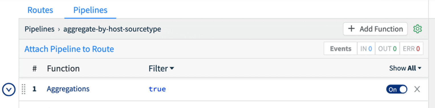
Let’s say that I have a new set of data I want to onboard. First, let’s setup an aggregation pipeline to give us some summary statistics. In the Cribl UI, we’re going to add a new pipeline, called aggregations. Click Pipelines > Add Pipeline > Create Pipeline. In Id, I called mine aggregate-by-host-sourcetype, but you can call yours whatever you want.
Now we’re going to add an aggregation function to our pipeline. Aggregation does a tumbling window aggregation of the data flowing through this LogStream pipeline, with user configured aggregations and groupings. For this use case, our aggregation needs are pretty simple. We want to count the number of events coming through this pipeline and we want to know the total bytes in the _raw field so we can estimate storage and licensing capacity consumption from a given sourcetype.
First, click Add Function, search for agg, and add the Aggregations function. We’ll leave Filter set to trueand the Time Window set to 10s. For this use case, 60s or longer would work fine and emit 6x less data, although the data for estimation is tiny even at 10s as we’ll see below. Next, we’ll add our Aggregates. Aggregates are another type of expression in Cribl, easily discoverable via typeahead in the UI, or you can view a full list in the docs. I add count(), so we’ll get a count of events, and sum(_raw.length).as('raw_length_sum'). You can see with this example, I’m chaining functions in the expression and the chained as() function renames the field. This is necessary since Splunk does not allow fields beginning with an _.
Next, I’m going to add my group by fields. For this use case, I want to group by host and sourcetype so I can get a view of the data coming in based on where it’s coming from and the type of data I’m working with. Lastly, I’m going to add some Evaluate Fields which will ensure my new aggregation events have the standard set of Splunk metadata. host and sourcetype come from the Group By Fields, so we need to add index and source manually. I set index to 'cribl' and source to 'estimation'. Note the ' in the value, as I want to express a string literal here rather than a field called cribl. source is optional, but it helps me easily query Splunk for this estimate records while keeping the sourcetype the same from the original data.
Hit Save, and now we have a pipeline which is aggregating all data coming through it by the host and sourcetype fields. We can validate this in Preview by running a capture. On the right, click Preview, then Start Capture. Capture data for sourcetype=='access_combined'. Hit save, and then in Preview, you’ll see a bunch of crossed out events. Turn off Show Dropped Events, then we’ll see only the aggregation events.
Installing the Pipeline as a Route
Now that we have a pipeline which will process data the way we want, we need to install a Route which will send data through that pipeline. From the pipeline we’re in, we can click Attach To Route which will bring us back to the Routes screen or just click the Routes tab. Click Add Route at the top, which will insert a new route at the bottom. Drag it up to the top, because we want to match events first. First we enter a name for the route, which I called estimate, and then we enter a filter condition. I want to estimate sourcetype access_combined, so I enter a Filter expression of sourcetype=='access_combined'. Note the two == and the ' indicating it’s a literal string. I select my aggregate-by-host-sourcetype pipeline and I choose to output it to Splunk.
One important concept here for our estimation use case is the concept of a Final route. In this route, I left Final set to yes, which means all events which match my Filter will go down that pipeline and be consumed by that pipeline. For our estimation use case, this is exactly what we want, as we don’t want the original data to go to the destination, only our aggregates. If we wanted to also process that data with another pipeline, we would set Final to no.
After installing the route, we should see the Event percentage increase from 0.000% up to some larger fraction. If we go back into the pipeline, we should also see the event counts increasing at the top of the pipeline. The large disparity in Event counts is exactly what we’re looking for. The output of the aggregation pipeline is a trickle of data compared to the original raw volume.
Using Aggregates in Splunk
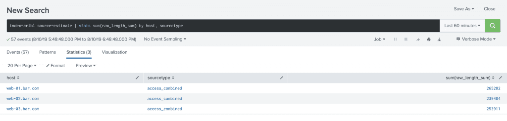
Analyzing the data in Splunk is easy. Every 10 seconds, Cribl outputs an event to Splunk which looks like it did in Preview up above. There will be a JSON document with a field count and a field raw_length_sum. In order to see how much data would have come in over a given period, simply run a search like index=cribl source=estimation | stats sum(raw_length_sum) by host, sourcetype.
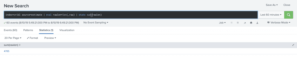
If you want to see how much data was consumed by the estimation records, a search like index=cribl source=estimation | eval rawlen=len(_raw) | stats sum(rawlen) will show you the size of the estimation records. It’s quite small.
Wrapping Up
Aggregates allow us to take very large data volumes, analyze them as they’re streaming, and output summary statistics to still get the value from the original signal while removing all the noise. If you have high volume log data sources like flows or web access logs, converting them to metrics can give you most of the value on a fraction of the data. These metrics can be sent also to a dedicated metrics store like Splunk, InfluxDB, Prometheus, or others for fast reporting and alerting.
There are a ton of use cases in addition to estimation: converting logs to metrics, monitoring data distribution across data nodes or indexers, summarizing data for fast reporting, and a myriad of others. LogStream gives users numerous techniques to maximize the value of their log streams: suppression and streaming deduplication, sampling and dynamic sampling, and aggregation. These techniques enable processing of data that has always been too expensive to store at full fidelity, and paired with our routing capabilities, allow users to manage their data based on what they can afford. Full fidelity can easily be shuffled off to cheap object storage with metrics going to a metrics store and a smart sample going to a log analysis tool.
We would love to help you get started with any of these use cases. If you have any questions, you can chat at us via the intercom widget in the bottom right, or join our community Slack! You can also email us at hello@cribl.io. We look forward to hearing from you!